A three-layer network was used, with 2x4x2 inputs going to a hidden layer of 3 tanh units and 1 output unit. Half-lives for averaging: U=5, V=500.
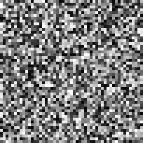
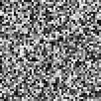
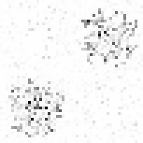
The inputs to the network are the following two binary images (no smoothing or normalisation of input patches):
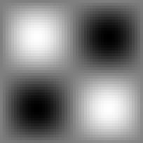
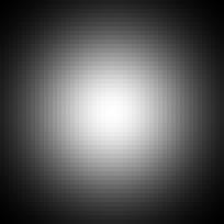
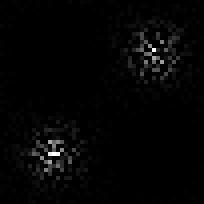
The product of the two patches in each image has an "egg-box" profile (shown on the left). Network performance after 200 epochs is shown on the right. Final correlation between desired and actual output is -0.994.

[All images here are jpegs which accounts for the poor quality on some of the graphs.]
Note this is a very low value of the merit function -- typically we used to see values of around 1.8 for the disparity test and around 0.9 for the feature orientation. [It is negative since we are taking logs and the value V/U has gone below 1.0.]
Inputs are just the binary values (no smoothing or normalisation of input patches):
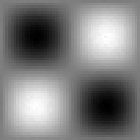
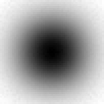
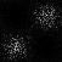
The product of the two patches in each image has a Gaussian profile (shown on the left). Network performance using the network trained on egg box data above is shown the right. Correlation between the two is -0.977, hence the network has generalised from the egg-box data to the gaussian data.
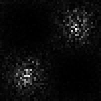
The network was also tested on another pair of inputs where z varied randomly over the image (inputs not shown). Correlation between the desired output (below left) and network output (below right) was -0.995.
In this case, the merit function reached a stable value of -0.8 after around just 10 epochs. When tested on the unseen Gaussian images, correlation was very high (-0.97).
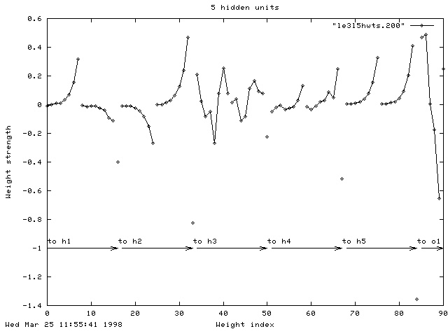
For each of the five hidden units (h1...h5) you see the connections to the eight inputs from the left patch, then the eight inputs from the right patch and then the bias unit. For the connections to the output unit (o1) you see the weights from the five hidden units and then the bias weight. The weights to the third hidden unit look quite strange, although the strength of the connection from h3 to o1 is almost zero so that unit is probably not being used.
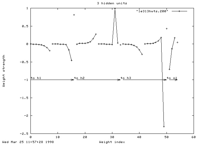
The network was also tested with three, rather than five, hidden units. Although the final correlation at the end of learning was high (0.972), it didn't generalise across to the test images very well (When tested on Gaussian data, r=0.800. However, when tested on the random data, r maintained a high value of 0.976).
See also adding numbers.