2 A Quantum Particle in One Dimension
There is much more to say about the basic postulates of quantum mechanics. However, rather than presenting the full mathematical framework up front, we’re instead going to explore a few simple examples of the Schrödinger equation. In doing so, we’ll build some intuition for how to think about the wavefunction and the various pieces of information that it encodes. Along the way, we’ll motivate how to think about physics in the quantum world.
A few of the steps in this section will involve something of a leap of faith as we try to elucidate the meaning of the wavefunction. In Section 3, we will return to the basic formulation of quantum mechanics where we will state the rules of the game more precisely and present a more complete description of the theory.
We will cut our teeth on quantum mechanical systems that involve a single particle moving in one spatial dimension. This means that the wavefunction depends on just a single variable (in addition to time) and the Schrödinger equation becomes
We will solve this equation for various choices of and interpret the results.
The Time Independent Schrödinger Equation
At first glance, the Schrödinger equation looks fairly daunting because it is a partial differential equation. In fact, there is a straightforward way to deal with the time variable. The idea is to look for separable solutions of the form
| (2.8) |
for some choice of frequency . Note that we have indulged in a slight abuse of notation, denoting both and with the same variable. In what follows, it will hopefully be clear which one we are talking about in any given circumstance. Where there is a possibility for confusion, we’ll keep the arguments explicit.
Because this is the way that we will solve all Schrödinger equations in these lectures, let us briefly return to the general case with
| (2.9) |
Plugging in the ansatz (2.8), we find ourselves having to solve
| (2.10) |
This is known as the time independent Schrödinger equation. If you really want to make a distinction, the original Schrödinger equation (2.9) is, of course, known as the time dependent Schrödinger equation. Here we’ll usually just refer to both as the Schrödinger equation unless there’s likely to be some confusion about which one we’re talking about.
The Schrödinger equation in the form (2.10) looks very much like the eigenvalue equations that we meet when working with matrices and this is a very good analogy to have in mind as we proceed. In all the examples that we study, we’ll see that there are solutions to (2.10) only for very specific values of . Furthermore, these special values of will have the interpretation of the possible energies of the system.
Separable solutions of the form (2.8) are sometimes referred to as stationary states and sometimes as energy eigenstates. They play a special role in quantum mechanics. One might worry that restricting attention to solutions of this kind is too restrictive, and that we are missing a whole bunch of other interesting solutions. In fact, as we go on we will see that all solutions can be expressed as linear combinations of different stationary states.
2.1 The Free Particle
Our first example is the simplest. We take a particle moving in one dimension in the absence of a potential
In this case, the time independent Schrödinger equation reads
| (2.11) |
All we have to do is solve this. The solutions are straightforward to write down: there is a different solution for every , given by
| (2.12) |
The eigenvalue in (2.11) is then given by
| (2.13) |
As we mentioned above, the value has the interpretation of the energy of the state . For now, take this as just one more postulate of quantum mechanics, perhaps one that has some justification given our earlier comments about the relationship between the energy and the Hamiltonian. We’ll revisit these postulates in Section 3.
If we do interpret (2.13) as the energy of the particle, we should probably compare it to our classical expectations. In the absence of a potential energy, there is only kinetic energy and this is given by
where is the momentum of the particle. Clearly this suggests that the momentum of the state (2.12) should be identified with
| (2.14) |
This is the correct interpretation. We will later see that (2.12) is a “momentum eigenstate”, which means that it is a state with definite momentum.
The wavefunction (2.12) can be viewed as a sum of sine and cos functions and describes a complex-valued wave of wavelength
| (2.15) |
Here the is needed because can have either sign, while the wavelength is always positive. The relationship (2.14) between the momentum and wavelength then becomes
In this context, is called the de Broglie wavelength of the particle. Any non-relativistic particle, with momentum , has an associated wavelength and, as we will see, in certain situations will exhibit wavelike properties. The more grown-up version of the de Broglie relation is (2.14) where is referred to as the wavenumber. However, it’s not unusual for physicists in general (and me in particular) to be sloppy and refer to as the momentum.
There is, however, an annoying subtlety that arises in this simplest example of quantum mechanics. The wavefunction (2.12) is not normalisable! If you integrate it you get
That’s bad! It means that we can’t actually think of as a state of our particle. What should we make of this?
This is a slippery issue, and one that doesn’t arise in many other situations. We will, ultimately, address this issue head on in Section 2.4 where wavefunctions like (2.12) will be too useful to ignore. But we will be best served if we first side step the problem and look at situations where it doesn’t arise.
2.1.1 A Particle on a Circle
One simple fix is to consider a particle moving on a circle of radius . The Schrödinger equation is still (2.10) and its solutions are still (2.12), but now there is the additional requirement that the wavefunction should be periodic, so that
Not all solutions (2.12) obey this requirement. We must have
This holds only for of the form
This is our first sign of the quantum in quantum mechanics. This word refers to the fact that certain quantities, which are always continuous variables in the classical world, can only take certain discrete values in this new framework. For the particle on a circle, we see that the momentum is quantised
| (2.16) |
as is the energy
The possible values of the momentum are split by . As the circle gets larger, the gap between the allowed momentum states becomes smaller. At some point, this will be experimentally indistinguishable from momentum taking arbitrary real values. Similar comments hold for the energy. The collection of all possible energies is known as the spectrum of the Hamiltonian.
As an extreme example, we don’t know if our universe is infinite or if it is finite, with a radius light years. If the latter is true, then you wouldn’t be able to travel with arbitrary momentum, but only very specific values finely graded by . Needless to say, we have no way of measuring momentum to an accuracy which can distinguish these two options.
Conversely, suppose that there are spatial dimensions in our universe beyond the obvious three that we see. If such dimensions exist, we need a reason why we’ve not observed them. One obvious possibility is that they wrap around to form a circle or some other compact space. In this case, the lowest energy wavefunctions simply spread uniformly around the extra dimension. If you want to move in the extra dimension, then you need a minimum amount of momentum and, correspondingly, a minimum amount of energy . If we can’t muster this minimum energy then we are unaware of these extra dimensions. But, ironically, we’re unaware of them because we inhabit them uniformly, rather than because we’re stuck at one point.
There are no pressing reasons to believe that extra dimension exist in our universe. Our best particle accelerators reach energies of around eV, also known as a TeV, and there is no sign of them knocking particles into the next dimension. This puts a limit on the size of these putative small extra dimensions of m or so. (To give you the fuller story, you really need relativistic dynamics by the time we get to these energies. The result is that the minimum momentum in the extra dimension requires energy , but the general conclusion remains unchanged.)
The discreteness in quantities like momentum and energy is one of the characteristic features of quantum mechanics. However, as the example above illustrates, there is no discreteness in the fundamental equations. Instead, the discreteness is an emergent phenomenon. The integers arise only when you solve these equations. In the current example, there is a nice intuitive explanation for how this arises: the only states that are allowed are those for which an integer number of de Broglie wavelengths fits nicely around the circle. Indeed, the quantisation condition (2.16) becomes
Finally, we can return to the normalisability issue that plagued our earlier example of a particle on a line. The wavefunction (2.12) is not normalised but, when viewed on a circle, it is at least normalisable. We have
which tells us that the correctly normalised wavefunction is
You can see that this doesn’t fare well if we try to return to a particle on the real line by taking . In this limit, the wavefunction becomes smaller and smaller in its attempt to remain normalised, until it vanishes completely.
2.1.2 The Infinite Potential Well
We get very similar physics by looking at a particle trapped in an infinite potential well of width . We can achieve this by setting
You may think that we’re no longer dealing with a free particle now that we’re subjecting it to an infinite potential energy. However, the effect of an infinite is very easy to deal with. The Schrödinger equation equation is
and if we’re looking for states with finite energy , then we must have in any region where . Intuitively this is obvious: the infinite potential is just a plot device that allows us to insist that the particle is restricted to lie in the region . Within this region, we again have our free Schrödinger equation
but now with the restriction that at the two ends of the interval and . The solutions are, once more, a restricted class of the wavefunctions.
To see the restriction in more detail, first recall that in our previous example the wavevector can take either sign. Moreover, and describe two different states; from (2.14) they correspond to a particle with positive or negative momentum. For the particle in the interval, we will consider the more general ansatz
now with . The requirement that tells us that , so the wavefunction must be of the form
The factor of in front simply changes the normalisation of the wavefunction and doesn’t affect the physics. Indeed, if we want the wavefunction to be normalised correctly, should take
| (2.17) |
But now we have to impose the requirement that the wavefunction vanishes at the other end of the integral, , or
The wavefunctions for the and 4 states are shown in Figure 8.
There is one slightly subtle difference from our previous example: in current case should be a positive integer, while for the particle on the circle it could have either sign. This is because reversing the sign of in (2.17) merely flips the overall sign of the wavefunction which, as we have seen, does not give a different state. This means that the and states are the same. Meanwhile, if you set , the wavefunction simply vanishes and and so the upshot is that we restrict to be a positive integer.
In this example, we again see that energy is quantised, taking values
| (2.18) |
This is very similar to the result of a particle on a circle.
What about the momentum? Recall our previous discussion: the state has momentum . But for the current example, we have (ignoring the normalisation) . This is the superposition of two states, one with momentum and the other with momentum . This means that these states do not have a well defined momentum! You can think of them as standing waves, bouncing backwards and forwards between the two walls but not going anywhere. We’ll become more precise about how to identify the momentum of a state as we go on.
The discreteness of energy levels in the infinite well has an important application, similar in spirit to the “extra dimension” story that we told above, but significantly less science fiction. Consider particles moving, as particles do, in three spatial dimensions. Suppose that you trap them in a well in one dimension, but still allow them to wander in the other two. Then, provided that you can restrict their energies to be small enough, the particles will act, to all intents and purposes, as if they’re really two-dimensional objects.
This is in sharp distinction to what happens in classical mechanics where the particles would move approximately in two dimensions but there would always be small oscillations in the well that can’t be ignored. However, the discreteness of quantum mechanics turns an approximate statement into an exact one: if the particle doesn’t have enough energy to jump to the state then it really should be thought of as a 2d particle. Of course, we can also restrict its motion once more and make it a 1d particle.
This may not seem like a big deal at this stage but, as we will learn in later courses, interesting things can happen in low dimensions that don’t happen in our 3d world. But these things aren’t mere mathematical curiosities but can be constructed in the lab using the method above. (If you want an example, in 2d — but not in 1d or in 3d — it’s possible for an electron to split into objects each carrying fractional electric charge . And this can be seen in experiments!)
2.1.3 The Gaussian Wavepacket
Let’s now return to the problem of a free particle moving on a line, with . Recall that the time dependent Schrödinger equation is
This is solved by the separable solution
for any choice of . In anticipation of what’s coming next, we’ve changed the notation to make it clear that both the wavefunction and the energy depend on the wavenumber , with the latter given by
The problem, as we’ve seen, is that is not a normalisable wavefunction on and therefore is an illegal state. However, that doesn’t stop us from taking superpositions of to build states that are normalisable. The most general superposition takes the form
| (2.19) |
for some function . Moreover, for each choice of , this wavefunction will solve the time dependent Schrödinger equation . This follows from a simple, yet important, observation about the general time dependent Schrödinger equation (1.1): it is linear. This means that if you find two solutions and that solve the Schrödinger equation, then their sum is guaranteed to solve it as well. This linearity of quantum mechanics is, like the Schrödinger equation itself, something that persists as we move on to more advanced topics. It is one of the very few ways in which quantum mechanics is simpler than classical mechanics.
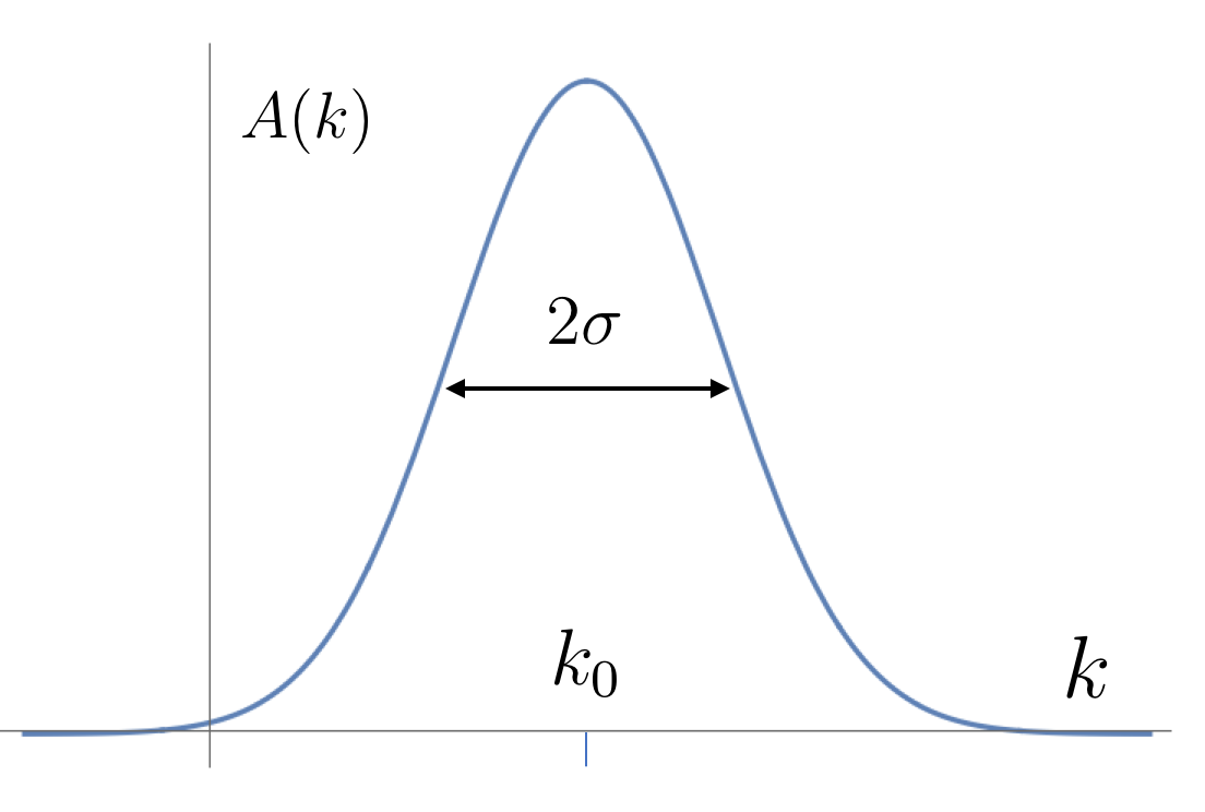
For our purposes, let’s consider a wavefunction built by taking
This is a Gaussian distribution over momentum states , centred around the wavenumber , with width . A sketch is shown to the right. The additional factor of is just a constant and only affects the normalisation of the wavefunction; we’ve included it so that things look simpler below.
When used to construct the linear superposition (2.19), the Gaussian distribution means, roughly speaking, that we include significant contributions only from wavenumbers that lie more or less within the window
| (2.20) |
Outside of this window, the coefficients drop off very quickly. What does the resulting wavefunction look like? We have
where, in the second line, we have simply completed the square and the various parameters are given by
| (2.21) |
At this stage, we have an integral to do. This is well-known Gaussian integral, with
This result holds for any and for any with . A quick look at the defined above confirms that we’re in business, and the final result for the wavefunction is
| (2.22) |
where the function is defined in (2.21). We see that the wavefunction also takes the form of a Gaussian, now in space, and with a time dependent width .
There’s a lot to unpack in this formula. First, note that the wavefunction is normalisable. (Although, as we shall see shortly, not actually normalised.) This follows from the fact that decays exponentially quickly as . So although we built the wavefunction from the non-normalisable, and hence illegal, waves (2.12) there’s nothing wrong with the end product. This is the first sign that we shouldn’t be so hasty in simply discarding the wavefunctions on the line. They may not be genuine states of the system, but they’re still useful.
The state described by (2.22) has neither definite momentum nor energy nor, indeed, position. This is actually the lot of most states. Moreover, the state does not take the simple separable form (2.8) of the stationary states that we’ve discussed until now. Indeed, the time dependence is fairly complicated. It turns out that one can construct all solutions of the Schrödinger equation through similar linear superpositions of stationary states. When, as in the present case, the stationary states are simply , the linear superposition is just the Fourier transform of a function. But it also holds in more complicated cases. This is why its sensible to solve the time dependent Schrödinger equation by first looking for solutions to the simpler time independent Schrödinger equation. We’ll address this further in Section 3.
Next, we can try to extract some physics from the state (2.22) which goes by the name of the Gaussian wavepacket. Clearly it describes a state that is fairly well localised in space. But, as time goes on, it becomes more and more spread out11 1 The Mathematica website has a nice demonstration of an evolving Gaussian wavepacket.. This is what happens to quantum probability if it is not trapped by some potential: it disperses. It is only the stationary states that have a definite energy and, correspondingly, the simple time dependence that stick in one place.
There is also something interesting in the size of the dispersion. Recall that we built the state by integrating over momentum modes in the window (2.20). We can think of this in terms of the variance, or uncertainty, of the wavenumber which we write as
where is an important mathematical symbol that means the thing of the left is roughly like the thing on the right. It’s useful in physics when trying to tease out some relation without bothering about all the details like annoying numerical coefficients. Meanwhile, the spread in position is determined by the function given in (2.21). It is at its minimum when , so we have
We see that the spread of the wavefunction in position space is inversely proportional to its spread in wavenumber or, equivalently, its spread in momentum . Multiplying these together, we get
This is our first glimpse at the famous Heisenberg uncertainty relation. You can localise a particle in space only at the expense of having a broad range of momenta, and vice versa. We’ll derive the proper mathematical expression of the Heisenberg uncertainty relation in Section 3.4.1.
This also gives us a new perspective on our original attempt at writing states as . These wavefunctions have a definite momentum, . But they are also spread out everywhere in space and this is what resulted in their non-normalisable downfall.
2.1.4 A First Look at Expectation Values
There is one thing that might still seem puzzling about our wavefunction
We constructed it by summing over states with different wavenumbers, but they were peaked around . And one might think that this should result in a particle moving with some average momentum . But it’s not obvious that our wavefunction is moving to the left or right in any way. In fact, pinning down its location is a little bit confusing because there’s the imaginary piece sitting in the exponent. How should we think of this?
To get a better sense of what’s going on, we should compute the probability density . At this point we should be more careful about the overall normalisation, so we introduce a constant that we’ll figure out later and write . We then have
| (2.23) | |||||
where you need a little bit of algebra to get to the second line. You can check that the probability is correctly normalised if we take . Importantly, the normalisation factor itself doesn’t depend on time. This had to be the case because we’ve constructed this wavefunction to obey the time dependent Schrödinger equation and, as we saw in Section 1.2.2, if you normalise the wavefunction at one time then it stays normalised for all times.
From the form of the probability (2.23), you can clearly see the growing width of the distribution, with
However, it is now also clear that the probability distribution doesn’t just sit at the origin and spread out, but instead moves. This follows because the dependence takes the form where the velocity is
If we think in classical terms, and define the momentum to be , then we have as expected.
There should be a more systematic way to extract this information about the momentum of a state, one that doesn’t involve staring at complicated formulae to figure out what’s going on. And there is. Our equation (2.23) is a probability distribution for the position of the particle. As with any probability distribution, we can use it to compute averages and variances and so on.
Given a probability distribution , with , the average of any function is given by
In quantum mechanics the average is usually called the expectation value and, as above, is denoted by angular brackets . We can then ask: what is the average position of the particle given the probability distribution (2.23)? We simply need to compute the integral
where, in the second line, we’ve shifted the integration variable to . We can now use the general result for Gaussian integrals,
| (2.24) |
where the second equality follows because the integrand is odd (and suitably well behaved at infinity). Using these, we get
showing, once again, that the wavepacket travels with velocity .
We could do further calculations to compute the average of any other function . But instead we’re going to pause and ask a different question. How do we compute the average momentum of the wavepacket?
At first glance, this might seem like an odd question. After all, we’ve just computed the velocity and so the average momentum is surely . However, in later examples things won’t be so straightforward and this is a useful place to pause and see what’s going on.
One reason this is an interesting question is because it gets to the heart of the difference between classical and quantum mechanics. In classical mechanics, the state of the system is determined by both and . But in quantum mechanics we have only the wavefunction, and this has to contain information about both position and momentum. So how is this encoded? This is one of the steps in this section that involves a leap of faith and no small amount of creativity.
In fact, we saw a hint of how to proceed back in the introduction. Recall that our Hamiltonian for a one-dimensional particle is
while, in classical mechanics, the energy of a particle is
This suggests a relationship between momentum and the act of taking a derivative
where I’ve picked the minus sign, as opposed to plus sign, because I’ve studied this course before. This is the clue that we need. Given a wavefunction , the momentum is encoded in how fast it varies in space. We can see this in the simple non-normalisable states where and is clearly bigger for higher momentum. In general, the correct relationship between momentum and the derivative manifests itself in the following formula
| (2.25) |
We’ll have a lot more to say about this in Section 3. For now, let’s just see what it gives for our Gaussian wavepacket. We have
where, after taking the derivative, the algebra needed to go from the first to the second line is identical to that in (2.23). Again shifting the integration variable to , we have
where, to get the final equality, we did the Gaussian integrals (2.24) and then used the expression for given in (2.21).
That was a fair bit of work just to get the answer that we expected all along: . As we go on, we’ll see that the expression (2.25) is the right way to think about the average momentum of any state.
2.2 The Harmonic Oscillator
The harmonic oscillator is the name given to a particle moving in a quadratic potential. In classical mechanics, the energy is
| (2.26) |
The classical equation of motion follows from the fact that energy is conserved, which means that or, equivalently,
The most general solution has the form and describes a particle bouncing backwards and forwards with frequency .
In this section we will look at the quantum harmonic oscillator. This means that we want to solve the Schrödinger equation with Hamiltonian
| (2.27) |
It’s difficult to overstate the importance of the harmonic oscillator in quantum mechanics. It is, by some margin, the single most important example that we will study. The reasons for this are twofold. The first is Taylor’s theorem: if you take any potential and expand close to a minimum then, at leading order, you will most likely find the harmonic oscillator. This means that small perturbations of more or less any system in Nature are described by the Hamitonian (2.27). (There are exceptions. Very occasionally, you might find a potential where the quadratic term vanishes, so , and you have to look at the next term in the Taylor expansion. This situation is rare but interesting.)
The second reason for the utility of the harmonic oscillator is more practical. Human beings are not particularly good at solving equations. This isn’t so apparent when you first learn theoretical physics because, quite reasonably, your teachers don’t want to stand up in front a classroom and continually repeat “yeah, we don’t know how to solve this one either”. Instead we shine a light on our successes. But as theoretical physics gets more advanced, these successes become harder and harder to find. At some point the only system that we can actually solve is the harmonic oscillator. Or, more precisely, things that can be made to look like the harmonic oscillator. The art of theoretical physics is then to make everything look like a harmonic oscillator. Take whatever you think is the coolest result in physics – maybe the Higgs boson, or some new material like topological insulators, or maybe gravitational waves or Hawking radiation. For all of them, the underlying theory is primarily to do with harmonic oscillators.
There are, it turns out, a number of different ways to solve the harmonic oscillator. In these lectures we won’t do anything fancy and just go ahead and solve the Schrödinger equation equation viewed as a differential equation.
2.2.1 The Energy Spectrum
Our goal is to find solutions to the time independent Schrödinger equation ,
| (2.28) |
Here the word “solution” means finding all normalisable that satisfy the Schrödinger equation and, for each one, the accompanying energy .
There are a bunch of constants sitting in (2.28) and life is simpler if we can just get rid of them. To this end, define
| (2.29) |
Then the Schrödinger equation takes the cleaner form
| (2.30) |
Before we get going, we can find one solution just by staring. This is the Gaussian wavefunction
| (2.31) |
The derivatives are and , so we see that this obeys the Schrödinger equation with (rescaled) energy .
Furthermore, it’s simple to see that all normalisable solutions should fall off in the same exponential fashion, with as . This follows from looking at the large behaviour of (2.30), where the term is necessarily negligible compared to the . This motivates the general ansatz
| (2.32) |
where we will shortly take to be a polynomial. Taking derivatives of this wavefunction gives and so the Schrödinger equation (2.30) becomes
| (2.33) |
You can check that this is indeed satisfied by our earlier solution (2.31) with . To find the general solution, we take the polynomial ansatz
Here is just a dummy summation index; do not confuse it with momentum! Plugging this ansatz into (2.33) gives a relation between the coefficients,
| (2.34) |
All we have to do is solve this simple recursion relation.
First note, that the recursion relation involves two independent sets of coefficients: with even, and with odd. These two sets don’t talk to each other and so we have two classes of solutions. We’ll see the interpretation of this shortly.
Next, let’s look at what happens for large . There are two options: either the recursion relation terminates, so that for all for some . Or the recursion relation doesn’t terminate and for all . We’re going to argue that only the first option is allowed. If the recursion relation keeps going forever, the resulting wavefunction will be non-normalisable.
Why is this? If the recursion relation doesn’t terminate then, for very large , we have . But this is the kind of expansion that we get from an exponentially growing function. To see this, look at
The appropriate recursion relation for this exponential function is then
The upshot of this argument is that, if the recursion relation (2.34) fails to terminate then, for large , the wavefunction actually looks like
The emergence of such solutions isn’t entirely unexpected. We know that, at large , both and are equally valid solutions. Our preference for the former over the latter is for physical reasons, but the power-law ansatz that we’re playing with has no knowledge of this preference. Therefore it’s no surprise that it offers up the solution as an option. Nonetheless, this doesn’t change the fact that it’s not an option we want to make use of. The wavefunctions are non-normalisable and therefore illegal. Moreover, unlike the more straightforward wavefunctions that we met in the last section, there’s no redemption for wavefunctions that grow exponentially quickly. They are not of interest and should be discarded.
All of which is to say that we should be looking for solutions to (2.34) for which the sequence terminates. This means that there must be some positive integer for which
| (2.35) |
But this is the spectrum of the theory that we were looking for! The allowed energy states of the harmonic oscillator take the form
Recalling the scaling (2.29), the energies are
| (2.36) |
All energies are proportional to , with the frequency of the harmonic oscillator. Furthermore the states are equally spaced, with
2.2.2 The Wavefunctions
It is not hard to get the wavefunctions. We simply work backwards from the result (2.35) to figure out all the earlier coefficients in the polynomial. We learn that the Gaussian wavefunction (2.31) that we guessed earlier is actually the lowest energy state of the system,
| (2.37) |
The lowest energy state in any system is called the ground state. Note that we also came across Gaussian wavefunctions (2.22) when discussing the free particle. In that context, they spread out over time. Not so here. The fact that the Gaussian is an energy eigenstate of the harmonic oscillator means that it has the simple time dependence of any stationary state. You can think of the wavefunction as pinned in place by the rising potential.
The next few (unnormalised) wavefunctions are
These, together with the Gaussian, are shown in Figure 9. In general, the functions are known as Hermite polynomials and have a number of nice properties.
We can now return to one issue that we left hanging. The recursion relation (2.34) does not relate with even to to those with odd. This manifests itself in the solutions above where the polynomials contain only even powers of or only odd powers of . Correspondingly, the two classes of solutions that we anticipated earlier are simply even or odd functions, with
There is a general lesson here. Whenever the potential is an even function, meaning , then the energy eigenstates will arrange themselves into even and odd functions. Underlying this is the concept of parity symmetry, which is the statement that the physics is unchanged under . We’ll make use of this idea of parity symmetry later in these lectures.
At first glance, the wavefunctions that we’ve found don’t seem to capture much of the familiar classical physics of a particle bouncing back and forth in a potential. Because they’re all stationary states, the time dependence is simply an overall phase in front of the wavefunction. You can compute the average position and momentum in any of the states above and you will find . In some sense, this is what you expect because it is also the average behaviour of the classical solution! Still, it would reassuring if we could see some remnant of our classical intuition in these wavefunctions.
A general property of quantum systems is that they tend to look more classical as you go to higher energies. For example, the discretisation effects may be less noticeable if they’re small compared to the overall energy of the system. For the harmonic oscillator, the wavefunctions for the and excited states are shown in Figure 10. Although it may not be obvious, some key elements of the classical trajectories can be seen hiding in these wavefunctions.
First, look at the way the wavefunction oscillates. We know that a free particle with definite momentum is associated to . The bigger , the smaller the wavelength, and the higher the momentum. In the wavefunctions shown in Figure 10, you can see that the wavelength of oscillations is much smaller near the bottom of the potential and then gets stretched towards the edges. This coincides with the classical expectation, where the particle is travelling much faster at the bottom of the potential and slows as it rises.
The way to quantify this idea uses a technique known as the WKB approximation. We’ll discuss this in more detail in the lectures on Topics in Quantum Mechanics, but here we just describe the basic idea which is enough to extract the physics that we care about. We write the Schrödinger equation equation as
The idea is that, for large , we might be able to think of the as roughly over some small region of . We then get two different kinds of behaviour: if then the wavefunction oscillates, approximately as for some . Alternatively, when , the wavefunction drops off as for some . The WKB approximation builds on this intuition by looking for solutions where itself is varies with , so . This, of course, is what’s seen in the wavefunctions plotted in Figure 10.
One consequence of this is that we expect that, as increases, the wavefunctions extend further out. Indeed, the wavefunction extends out further than the wavefunction. Mathematically this follows simply because there are higher powers of in the polynomial . The kind of ideas sketched above can be used to show that, for large , the final turning point of the wavefunction occurs at
This is precisely the turning point of the classical particle, where the kinetic energy in (2.26) vanishes.
Finally, look at the overall envelope of the wavefunction, a curve that peaks at the edges and dips in the middle. This is telling us that if you do a measurement of a particle in this high energy state, you’re more likely to find it near the edges than near the origin. But this, too, is the same as the classical picture. If you take a photograph of a ball oscillating in a harmonic potential, you’re most likely to catch it sitting towards the end of its trajectory, simply because it’s going slower and so spends more time in those regions. Conversely, the ball is less likely to be caught as it whizzes past the origin. This is, again, captured by the form of the wavefunction. We see that the quantum world is not completely disconnected from the classical. You just have to know where to look.
2.3 Bound States
Any potential that rises indefinitely at infinity will, like the harmonic oscillator, have an infinite collection of discrete allowed energies. In this section (and the next) we will look at a slightly different class of potentials, those which asymptote to some constant value
The value of the constant doesn’t matter; it just shifts the overall energies. For this reason, we may as well just set it to zero and consider potentials that asymptote to as . An example of such a potential is shown in the figure.

In fact there are a whole bunch of subtleties here to entrap the unwary. These relate to the question of how fast the potential asymptotes to zero. At this stage these subtleties are just an annoyance so we’ll assume that the potential falls off suitably quickly (for example, an exponential decay will certainly be fine).
Now we want to ask: what are the solutions to the Schrödinger equation
| (2.38) |
We can start to address this by looking at the form of the solutions as where the Schrödinger equation reduces to that of a free particle:
There are two qualitatively different kinds of solution to this equation:
-
•
Scattering States: The solutions with energy are characterised by and take the form
As we saw in Section 2.1 these states are non-normalisable and this remains true here. We’ll see what role they play in the next section where we will learn about scattering.
-
•
Bound States: The solutions with energy are characterised by and take the form
We didn’t even consider such wavefunctions when we discussed the free particle because they’re obviously badly non-normalisable. For example, we could set so that the wavefunction decays nicely as , but then it will blow up at .
However, it’s possible that we may be able to find good wavefunctions with this asymptotic form when we solve the full Schrödinger equation (2.38). For the state to be normalisable we would require that it decays at both ends, with
Note that to solve the Schrödinger equation we must have the same value of in the exponent on both sides to ensure that the solution has constant . Such wavefunctions are called bound states because they are necessarily trapped somewhere in the potential. As we will see, they occur only for very specific values of .
In the rest of this section, we will study a couple of simple potentials to get some intuition for how and when bound states occur. This will also provide an opportunity to address a couple of technical mathematical points that arise when solving the Schrödinger equation.
2.3.1 A Finite Potential Well
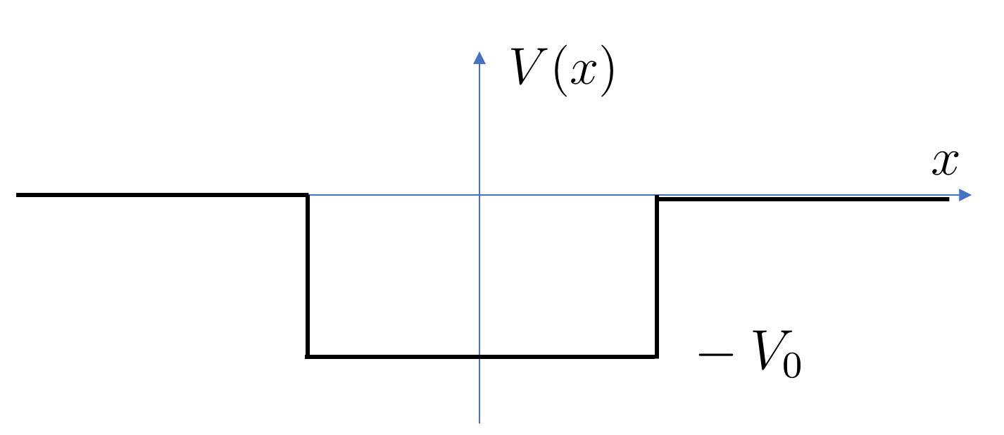
Our first example is the potential well of the form
| (2.39) |
It’s not difficult to see that there are no bound states if . We will take , so the potential is a dip as shown in the figure.
Clearly the potential is discontinuous at and this raises the question of what kind of wavefunction we should be looking for. The answer is that itself should be continuous, as too should . But inherits the discontinuity of the potential.
To see the statements above, first integrate the Schrödinger equation (2.38) over a small interval at ,
Although is discontinuous at , it is finite. This means that the integral on the right-hand side vanishes as we take limit , telling us that is continuous at . But if is continuous then so too is itself. Returning to the Schrödinger equation (2.38), we then see that the discontinuity in can only show up in the second derivative .
Now our strategy for solving the Schrödinger equation is clear: we find solutions inside and outside the well and then patch them together, making sure that both and are continuous at the join.
Before we proceed, there is one last idea that will make our life easier. This is the idea of parity, which comes from the observation that the potential is an even function with . This means that all solutions to the Schrödinger equation will be either even functions or odd functions. (We saw this in the example of the harmonic oscillator.) To see why this is necessarily the case, first note that if solves the Schrödinger equation for some value of , then so too does . Under the assumption that there aren’t two different wavefunction with the same energy (a so-called non-degenerate spectrum), we must have
for some . But we have
which tells us that , corresponding to either odd or even wavefunctions. (It’s possible to extend this proof even in the case of degenerate spectra but this won’t be needed for the examples that we’ll consider here.)
As we’ll now see, knowing in advance that we’re looking for even or odd solutions to the Schrödinger equation greatly simplifies our task of finding solutions. We’ll look for each in turn.
Even Parity Wavefunctions
Let’s start by taking the even parity case. We’re looking for bound state solutions which, outside the potential well, must take the form
| (2.40) |
Here is simply a normalisation constant. Our real interest is in the possible values of since these will determine the energy of the bound state .
Inside the potential well, the Schrödinger equation reads
This is, of course, once again the Schrödinger equation for a free particle, just with shifted energy. As before, there are two kinds of solutions:
-
•
Solutions with have wavefunctions .
-
•
Solutions with have wavefunctions .
It turns out that the former solutions are the ones of interest and all our bound states will have energies . This is perhaps not surprising give that is the lowest value of the potential.
Because we’re looking for parity even solutions, we should consider or,
| (2.41) |
where is again a normalisation constant and is, like , related to the energy, now with
| (2.42) |
Our next step is to patch the exponentially decaying solutions (2.40) outside the well with the oscillatory solution (2.41) inside the well. Because both solutions are even functions, we only have to do this patching once at ; the solution will then be automatically patched at as well. We have
There is no simple solution to this transcendental equation, but it’s not difficult to understand the property of the solutions using graphical methods. In Figure 11 we first plot the graph in blue, and then superpose this with the circle
shown in red. We restrict to the range as befits our normalisable wavefunction. We get a solution whenever the red curve intersects the blue one. As expected, there are a only discrete solutions, happening for specific values of . Moreover, there are also only a finite number of them.
We see that the first solution is guaranteed: no matter how small the radius of the circle, it will always intersect the first blue line. However, the number of subsequent solutions depends on the parameters in the game. We can see that the number of solutions will grow as increase the depth of the well, since this increases the radius of the red circle. The number of parameters will also grow as we increase the width of the well; this is because the separation between the blue lines is determined by the divergence of the tan function, so occurs when . As we increase , keeping fixed, the blue lines get closer together while the red circle stays the same size.
We can be more precise about this. From the graph, the crossing occurs somewhere in the region
giving an estimate of energy of the
In the limit of an infinite well, we have so the red circle becomes infinitely large, intersecting the blue lines only asymptotically where . Clearly all energies descend to in this limit, but we can instead measure energies with respect to the floor of the potential. We then get
But we’ve met this result before: it coincides with the energy spectrum (2.18) of a particle in an infinite well. (To see the agreement, we have to note that and, furthermore, remember that we have restricted to even parity states only which is why we’ve got only odd integers in the numerator.)
There is one last mild surprise in our analysis. All our bound states have energy
This is what we would expect for a classical particle, trapped inside the well. The quantum novelty is that the wavefunction itself is not restricted only to the well: it leaks out into the surrounding region , albeit with an exponentially suppressed wavefunction (2.40). This means that there is some finite probability to find the particle outside the well, in a region that would be classically inaccessible.
Odd Parity Wavefunctions
We can easily repeat this analysis in the case of odd parity wavefunctions. We’re now looking for bound state solutions which, outside the potential well, takes the form
Meanwhile, the odd parity wavefunction inside the well is
Patching these two solutions at gives
which now gives us
| (2.44) |
Once again this should be solved in conjunction with (2.42). Once again, graphs are our friend. The graph of (2.44) is shown in blue in Figure 12, while the circle corresponding to (2.42) is shown in red.
This time we see that there is no guarantee that a solution exists. The first blue line emerges from the axis at . The red circle intersects this first line only if
| (2.45) |
This means that the first parity odd solution exists only if the potential is deep enough or wide enough.
We can also see the solutions that were previously missing as we take . The divergences in the blue lines now occur at for any . Measured above the floor of the potential, the energies then become
where now we see that there are only even integers in the numerator.
2.3.2 A Delta Function Potential
As our second example, we will consider a potential that is, at first glance, slightly odd: a delta function sitting at the origin
for some constant . Recall that the delta function isn’t a real function, but a distribution satisfying
You can think of as an infinitely narrow, but infinitely long spike localised at the origin. You might think that it’s not particularly realistic as a potential, and there is some merit to that. But there are situations – such as impurities in solids – where the exact form of the potential is complicated and most likely unknown and it is useful to have a simple toy model that can be easily solved. This is what the delta function offers.
The discontinuity in the delta function is significantly more extreme than that of the finite potential well and, once again, we’re going to have to understand how to deal with it. Our strategy is the same as before: we take the Schrödinger equation as the starting point and see what the potential means for the wavefunction. To start, we integrate the Schrödinger equation over a small region around the origin
This time the right-hand side isn’t so innocent. While the term simply vanishes in the limit , the delta function doesn’t. We then find
| (2.46) |
We learn that the delta function leaves its imprint in the derivative of the wavefunction, and must now be discontinuous at the origin. The wavefunction itself, however, should be continuous.
This is all the information that we need to find a bound state. Away from the origin, the negative energy, normalisable solutions of the Schrödinger equation are simply
for some . Note that we’ve chosen normalisation factors that ensure the wavefunction is continuous,
However, the presence of the delta function means that the two solutions must be patched together with a discontinuity in the derivative
This should be identified with the discontinuity (2.46) giving the result that we need.
We learn that the negative-valued delta function has just a single bound state with energy
| (2.47) |
This calculation also makes it clear how the presence of a potential can change the asymptotic behaviour from as to as . The delta function does this all in one go, but can only achieve the feat for a very specific value of . More general potentials flip the sign of the exponent more gradually, but again can only do so for specific values of , leading to a (typically finite) discrete collection of bound states.
2.3.3 Some General Results
There are a number of simple, but useful, statements that we can prove for bound states in any 1d potential . These results hold for the two different kinds of potentials that we’ve discussed so far, namely
-
•
Potentials, like the harmonic oscillator, that diverge asymptotically so that as . These will have an infinite number of normalisable states that decay exponentially quickly as . In this case, we usually take and the states have energy .
-
•
Potentials, like the finite well, that asymptote to some constant which we can take to be as . As we’ve seen, these will have a finite number of bound states that decay exponentially, all of which have .
In what follows, we’ll refer to both kinds of states as bound states.
Claim: The spectrum of bound states is non-degenerate. This means that there aren’t two distinct wavefunctions with the same energy.
Proof: Suppose the converse is true, meaning that both and have the same energy so that
Consider the Wronskian,
This has the property that it is constant in space, as we can see by taking a derivative and using the Schrödinger equation
For normalisable states, we know the value of the Wronskian as : there we have , and so . Hence we must have everywhere. This means that, at any finite with , , we have
for some constant . But any two wavefunctions related by a constant correspond to the same state. This means that the spectrum is non-degenerate.
Note that the argument above fails for the non-normalisable momentum states since these are nowhere vanishing. And, indeed, such states are typically degenerate with and having the same energy.
Claim: The bound state wavefunctions can always be taken to be real.
Proof: If obeys the Schrödinger equation then so too does . We can then invoke the proof above to find for some constant . Taking the modulus square tells us that , so is a phase: . Now we can define and, as the name suggests, this is real. To check this, look at .
Claim: The ground state has no nodes. This means that except when .
Semi Proof: We’re running very slightly ahead of ourselves in attempting to prove this statement, but we’ve got just enough in place to give the gist of the proof, if not the full rigorous version. Suppose that you have a guess at the ground state wavefunction , but where , for some finite . We’re going to show that it’s always possible to construct a new state with lower energy.
In fact, that last statement is almost true. What we’re actually going to show is that it’s always possible to construct a new state with lower average energy. Following our discussion in Section 2.1.4, the average energy of any normalised, real state is
where, in the second line, we’ve integrated by parts and thrown away the boundary term because we’re dealing with normalisable states. The expression for the average energy should be plausible given our earlier result (2.25) for the average momentum. We will make it more precise in Section 3.3 when we discuss more about expectation values. For now, we will take it as given.
Now consider the state . The derivative is ill-defined any point where , but this doesn’t affect the average energy since it happens at a set of measure zero in the integral. This means that has the same average energy as . But now we can smooth out the cusp so that the derivative is smooth everywhere. Furthermore, in the region near the cusp, the derivative will be smaller after smoothing, which means that will also be smaller. This is how we lower the energy of the state.
Some fiddly mathematical analysis issues aside, there is one statement that we need to complete the proof. If the true ground state energy of the system is , then the average energy of any state is , with equality only for the ground state. This is intuitive and not too difficult to prove. It’s known as the variational principle in quantum mechanics and has quite a few applications. You can read more about this in the lectures on Topics in Quantum Mechanics. This variational principle now ensures that the initial guess with a node cannot be the true ground state of the system.
Claim: The excited state has nodes, i.e. distinct places where .
No Proof: This is significantly harder to prove and we won’t do it here. Note, however, that you can see the patten of increasing nodes in both the infinite well potential and the harmonic oscillator (and, if you work harder, the finite well potential).
2.3.4 The Double Well Potential
There is a particularly interesting system that we can’t solve exactly but can use the results above to get a feeling for the qualitative physics. This is the double well potential, which is the name given to any function that takes the shape shown in Figure 13.
Classically, the system has two ground states, corresponding to the two minima of the potential. The question is: what happens to a quantum particle placed in this potential?
We could focus attention near one of the minima, say the one on the right . If we expand the potential about this point, we have
For small , this looks just like the harmonic oscillator that we discussed in Section 2.2. Indeed, as we stressed back then, one of the reasons that the harmonic oscillator is so important is that it is the first approximation to almost all potentials when expanded about their minima.
We might reasonably think that we can import our understanding of the harmonic oscillator to understand what’s going on in this case. In particular, the ground state of the harmonic oscillator is a Gaussian (2.37),
where is a length scale determined by the mass of the particle and . The wavefunction is sketched in orange in the figure below. A first guess might be that this provides a good approximation to the ground state of the double well potential.
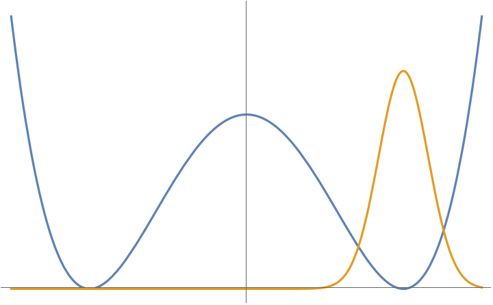
The trouble is, of course, that this guess runs afoul of the theorems above. In particular, it’s not unique. There is an equally good candidate localised around the left-hand minimum. If we assume that the potential is symmetric, so , then the other candidate ground state is
This looks the same as , but now peaked around the left-hand minimum.
What to do? Our analysis of the harmonic oscillator suggests that both of these should (at least for suitably chosen parameters) be good approximations to the ground state but they can’t both be the ground state.
The right way to proceed is to take linear superpositions of these states. Indeed, we saw earlier that for an even potential , all energy eigenstates are either odd or even functions. This tells us that the true energy eigenstates should be closer to
Furthermore, we know that the ground state has no nodes. This means that must be the approximation to the ground state while , which has a single node, should be the first excited state. Note the energy of is (again for suitably chosen parameters) expected to be much closer to than to the excited states of the harmonic oscillator around either vacuum. The two states are shown in Figure 15.
There is some striking physics that emerges from these simple considerations. Suppose that we put the particle in one of the wells, say the right. Classically the particle would stay trapped in that well provided that it’s kinetic energy wasn’t sufficient to get up and over the barrier in the middle. But that’s not what happens in the quantum world. Instead, the particle will lower its energy by sitting in a superposition of states like . Even if the particle does not have sufficient energy to get up and over the barrier it will, in time, leak through the barrier and have equal probability to be in either well. This phenomenon is known as quantum tunelling. We’ll see another manifestation of it in the next section.
2.4 Scattering
The basic principle behind scattering is simple: you take a particle, throw it at an object, and watch as it bounces off. Ideally, you can then use the information about how it bounces off to tell you something about the object in question.
In this section, we’re going to set up the basics of scattering in quantum mechanics. We will only solve some very simple situations and our goal is to continue to build intuition for how quantum particles behave.
Our set-up is the same as in Section 2.3. We have some potential that is localised in space and asymptotes suitably quickly to
| (2.48) |
In the last section, we understood that such potentials typically have some finite number of negative energy bound states, trapped in the potential. Here we instead ask: what happens if we stand far from the potential and throw in a quantum particle. Will it bounce back, or will it pass through the potential? Or, this being a quantum particle, will it do both?
Our first task is to set up the problem mathematically. One approach would be to construct a wavepacket, localised in space far from the potential, and send it moving towards the region where . This has the advantage that the wavepacket gels nicely with our classical expectation of a particle. It has the disadvantage that it is mathematically challenging. As we’ve seen, the wavepacket solution (2.22) is fairly complicated even for a free particle and becomes much more so in the presence of a potential.
Instead we’re going to take a different path. This involves resurrecting the wavefunctions of the form
for some constant . Recall that these have definite momentum , but are not valid states of the system because they are not normalisable. This last statement is doesn’t change if we work in the presence of a potential satisfying (2.48).
However, it is possible to endow wavefunctions of this kind with a different interpretation. Rather than thinking of them as quantum probabilities for a single particle, we will instead consider them as describing a continuous beam of particles, with the “probability density”
now interpreted as the average density of particles. To reinforce this perspective, we can compute the probability current (1.6) to find
| (2.49) |
where this last expression has the interpretation of the average density of particles multiplied by their velocity or, alternatively, as the average flux of particles.
There is a lot to say about scattering in quantum mechanics and the later lecture notes on Topics in Quantum Mechanics have a full chapter devoted to scattering theory. One of the highlights is understanding how we can reconstruct the spectrum of bound states of the potential by standing at infinity, throwing in particles, and looking at what bounces back. Here we will restrict ourselves to just two simple examples to build more intuition about the wavefunction and what it can do.
2.4.1 A Step Potential
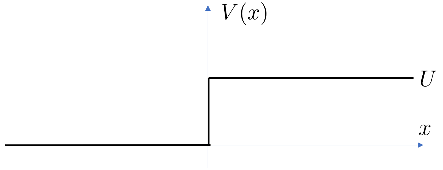
Our first potential is a step function
We will throw a particle – or more precisely a beam of particles – in from the left and see what happens. Our expectation would be that the beam will bounce back if the energy of the particles is less than , while if the energy is it should presumably fly over the small step without noticing. For energies that are just slightly greater than , something more interesting might happen.
Let’s now see how to set up the problem. We want to find a solution to the Schrödinger equation which includes a component at corresponding to an ingoing beam of particles,
with the density of the beam. We should also remember to take since this tells us that the initial beam is travelling to the right and will hit the potential. Clearly the energy of the particles in the beam is
However, the solution that we’re looking for will include a part of the wavefunction that bounces off the step and returns to , but with opposite momentum. In other words, we really want to look for solutions with the property
| (2.50) |
Note that the ingoing wave and the outgoing wave must have the same energy so this wavefunction is a solution of the Schrödinger equation. However, the densities of the beams can differ and, in general, we would expect telling us that not everything bounces back.
Although we set up the solution (2.50) as the boundary condition at , the fact that the potential vanishes means that this solution holds for all . It only changes when it encounters the step.
Next we look in the region where the potential energy is . Because the potential is constant, the general solution here is straightforward and given by
| (2.51) |
where, to solve the Schrödinger equation , the wavenumber is given by
| (2.52) |
Note that if the energy of the incoming beam is bigger than the step, , then is real. If, however, the energy isn’t big enough to get over the step, , then is imaginary. As we go on, we’ll understand how to think of an imaginary momentum.
At this stage, we need to think again about the physics. Suppose first that and so is real. Then the first term in (2.51) has the interpretation of an outgoing wave moving to the right, while the second term has the interpretation of a left-moving incoming wave, sent in from . But we didn’t send anything in from that end! Only from the end. That means that we should look for solutions with .
We reach the same conclusion if the beam had energy , in which case for some . In this situation, the is non-normalisable at and so should be discarded.
In either case, the upshot is that we’re looking for solutions of the form
| (2.53) |
Now we patch. We learned how to do this in the previous section: both and should be continuous at . This gives two conditions.
Recall that determines the density of the original, incident beam while and determine the densities of the reflected and transmitted beams respectively. We can solve the equations above to get expressions for the latter in terms of the former
| (2.54) |
We can view these in terms the particle flux defined in (2.49). For the original, incident beam we have
We’ve learned the flux in the reflected beam is
where, by convention, this reflected flux is taken to be positive. Meanwhile, the transmitted flux is
Let’s now think about how to interpret these results. We start with the case so that is real. This means that the particles aren’t forbidden from crossing the step on energetic grounds. But what do they do?
The answer to this is best seen by looking at the ratios of fluxes. We define
| (2.55) |
and
| (2.56) |
These are known as the reflection and transmission coefficients. They tell us what fraction of the incident beam is reflected and what fraction makes it over to the other side. Or, since we’re dealing with quantum mechanics, they tell us the probability that a particle is reflected or transmitted.
As a quick sanity check, note that
This is the statement that we don’t lose any of the beam. Nothing gets trapped at the step.
The result continues to hold for any potential. In particular, if you scatter a quantum particle off the kind of finite well potential that we discussed earlier, then we get , telling us that everything either bounces back or passes through. This means, in particular, that quantum golf is a rubbish game. The ball can’t drop into the hole and stay there because bound states necessarily have while our beam has . Anything that goes in must come out.
Although the expressions (2.55) and (2.56) are fairly straightforward when written in terms of and , we should really think of them just as a function of the incoming momentum , with determined in terms of by (2.52). You can quickly convince yourself that the formulae look much more complicated when written solely in terms of . But we can see that the physics sits well with our basic intuition. In particular, when , the outgoing momentum and so we see that
This makes sense: if the particle barely has enough energy to make it up and over the barrier then it is simply reflected back.
We still have one question left: what happens when the energy , so the particle can’t make it over the barrier. The key piece of physics can be seen in the wavefunction (2.53) which, for is
| (2.57) |
Our expression for given in (2.54) still holds, but with where . This, then, is the meaning of imaginary momentum: it tells us that the wavefunction decays exponentially inside the barrier. In contrast to classical mechanics, there is some non-negligible probability to find the particle a distance inside the barrier but beyond this point, the probability drops off quickly.
The calculation that we did previously only changes when we compute the fluxes. A wavefunction that drops off exponentially like (2.57) has vanishing current . It’s not transporting anything anywhere. The upshot is that when the energy is below the barrier height. You can check that, correspondingly, : everything bounces back.
2.4.2 Tunnelling
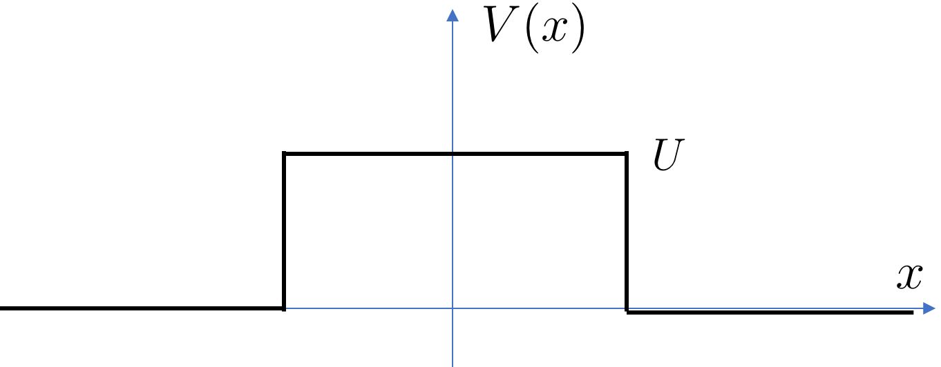
Our next example is a finite potential barrier, like a bump in the road
where . This is mirror of the finite well (2.39) whose bound states we studied earlier.
By now we know what to do: we write down solutions to the free Schrödinger equation in each region and patch at the join. We’re going to be interested in situations where the energy , which means that a classical particle would just bounces back. The question is: does a quantum particle with such low energy make it through the barrier?
Following our earlier discussion, we look for solutions of the form
Note that we’ve set the density of the incoming beam to unity, as seen in the term in the first line. This is in anticipation that this will drop out of the things we want to calculate, like and , and so it’s not worth keeping the extra baggage in the equations. The two exponents in the wavefunction are given by
| (2.58) |
Both are positive. The matching conditions at are
Meanwhile, the matching conditions at are
We have four equations. Our goal is to solve for in terms of and , since this will tell us the transmitted flux. It’s straightforward, if a little tedious. Here’s some handholding to help you along your way. First use the second pair of equations to write
| (2.59) |
Next, use the first pair of equations to write
We now substitute the expressions (2.59) into and in the equation above. A little bit of algebra then gives
| (2.60) |
We want to compute the transmission probability which, in this case, is just
Using (2.60), we get
| (2.61) | |||||
We see that there is a non-vanishing probability that the particle makes it through the barrier and over to the other side, even though a classical particle wouldn’t be able to do so. This is another manifestation of quantum tunelling.
To get some feel for the equation (2.61), let’s look at the extreme case of a very low energy particle. Low energy means , where “something” has to have the dimensions of energy. Some dimensional analysis shows that the requirement is
So the low energy limit is the same as the limit of a wide barrier. In this regime, the function in the denominator dominates. Written as a function of the incoming energy , transmission probability then becomes
where the exponent is multiplied by , with both and viewed as functions of the energy using (2.58). The key feature, however, is the exponential suppression of the probability. This is characteristic of tunnelling phenomena.
A very similar effect is at play in radioactive decay. In, admittedly rather simplified models, an alpha particle can be thought of as trapped inside the nucleus by a finite, but large potential energy barrier. A classical particle would be consigned to rattle around in the nucleus forever; a quantum particle can, with some exponentially suppressed probability, tunnel through the barrier and out the other side. The small probability manifests itself in the long lifetime of many unstable nuclei.