4 A Quantum Particle in Three Dimensions
We will now continue our explorations of the Schrödinger equation, this time focussing on a quantum particle moving in three dimensions, described by the Hamiltonian
where
Throughout this section, we will focus on a central potentials, with
These are both the simplest potentials to study and, happily, the kinds of potentials that are most useful for physics.
It’s worth recalling how we approached such potentials when we first met them in Classical Mechanics. In that context, everything became easier once we made use of the angular momentum vector
This is a conserved quantity in a central potential. To see this we just need to note that is parallel to and is parallel to . This latter fact follows from the classical equation of motion with the observation that is parallel to for a central potential. We then have
When solving central body problems in classical mechanics, we use the conservation of angular momentum twice. First we use the fact that the direction of is fixed to reduce the problem from 3d to 2d since the particle only moves in the plane . Later we use the fact that the magnitude is fixed to reduce the problem to motion in the radial direction. Then we solve what is essentially a 1d problem.
In this section we will see that a similar strategy works for quantum mechanics. The Schrödinger equation
is a partial differential equation. By the time we get to grips with angular momentum, it will be an ordinary differential equation of the same kind that we solved when considering a particle moving in one dimension.
4.1 Angular Momentum
The angular momentum operator is
In components, with , this means
Alternatively, these can be summarised in index notation as
It’s not hard to check that the angular momentum operators are Hermitian. Indeed, this really follows immediately from the fact that both and are Hermitian.
4.1.1 Angular Momentum Commutation Relations
The three angular momentum operators do not mutually commute. They obey the relations
| (4.84) |
From a physics perspective, this means that a quantum particle cannot have a well defined angular momentum in all three directions simultaneously! If, for example, you know the angular momentum then there will necessarily be some uncertainty in the angular momentum in the other two directions.
Although it goes beyond the scope of this course, I should point out that the commutation relations (4.84) are very famous in mathematics and appear in many places that have nothing to do with quantum mechanics. These equations define what mathematicians call a Lie algebra, in this case the algebra . It is very closely related to the group of which, in turn, is almost (but not quite!) the same thing as the group of rotations . In some sense, the commutation relations (4.84) distill the essence of rotation. The “almost but not quite” of the previous sentence opens up a number of weird and wonderful loopholes that the quantum world exploits. (Like, for example, the fact that there are particles called fermions that don’t come back to themselves when rotated by .). We discussed some of these issues briefly when exploring special relativity in the lectures on Dynamics and Relativity and we’ll meet them many more times in later courses.
Let’s prove the commutation relations (4.84). It will suffice to prove just one case, say
| (4.85) |
To check this, we recall that operator equations of this kind should be viewed in terms of their action on functions and then just plug in the appropriate definitions,
A little algebra will convince you that nearly all terms cancel. The only ones that survive are
Because this holds for all , it is equivalent to the claimed result (4.85). The other commutation relations (4.84) follow in the same vein.
Total Angular Momentum
We can also look at the magnitude of the angular momentum. It’s more useful to look at the rather than . This is associated to the total angular momentum operator
This is again a Hermitian operator. It commutes with all ,
| (4.86) |
This is important. As we saw above, quantum mechanics doesn’t allow us to assign simultaneous values to the angular momentum in all directions. However, a quantum state can have a specific total angular momentum – meaning that it is an eigenstate of – and also a specific value of angular momentum in one chosen direction – meaning that it is also an eigenstate of, say, .
To prove (4.86) we will first need a simple lemma. For any operators and ,
| (4.87) |
To prove this, we start from the right-hand side and expand out
We now just use this result repeatedly to prove (4.86). We want to show that, for example,
The first of these is trivial: all operators commute with themselves so . Using (4.87), the next two can be written as
| (4.88) | |||||
where, to get to the second line, we’ve used the commutation relations (4.84). We also have
| (4.89) | |||||
Adding (4.88) and (4.89) gives us the result (4.86) that we wanted.
Angular Momentum in a Central Potential
In classical mechanics, angular momentum is only useful when we have a central potential
Only in this case is angular momentum conserved.
The corresponding statement in quantum mechanics is that, for a central potential, we have
| (4.90) |
Again, this is important. It means that, for eigenstates of the Hamiltonian, total angular momentum and angular momentum in one chosen direction will be shared. A quantum particle can have simultaneous values for all three of these quantities. As we move forward, this is the result that we will allow us to solve the 3d Schrödinger equation.
Before we can do that, we first have to prove (4.90). It follows from some straightforward algebra that is very similar in spirit to what we’ve done so far. You can first show that
From this, it’s a small step to show that
But this is all we need. The Hamiltonian for a central potential is a function only of and ,
where . So we’re guaranteed to get . Since the Hamiltonian commutes with each angular momentum operator, it also commutes with the total angular momentum operator .
The upshot of this analysis is that a particle moving in a central potential can sit in simultaneous eigenstates of three operators, which we usually take to be:
The associated eigenvalues are energy, total angular momentum, and the angular momentum in the direction. In what follows, all energy eigenstates are labelled by these three numbers.
Note also, that this is the maximum set of mutually commuting operators. For a generic central potential , there are no further operators lurking out there that also commute with these three.
4.1.2 The Eigenfunctions are Spherical Harmonics
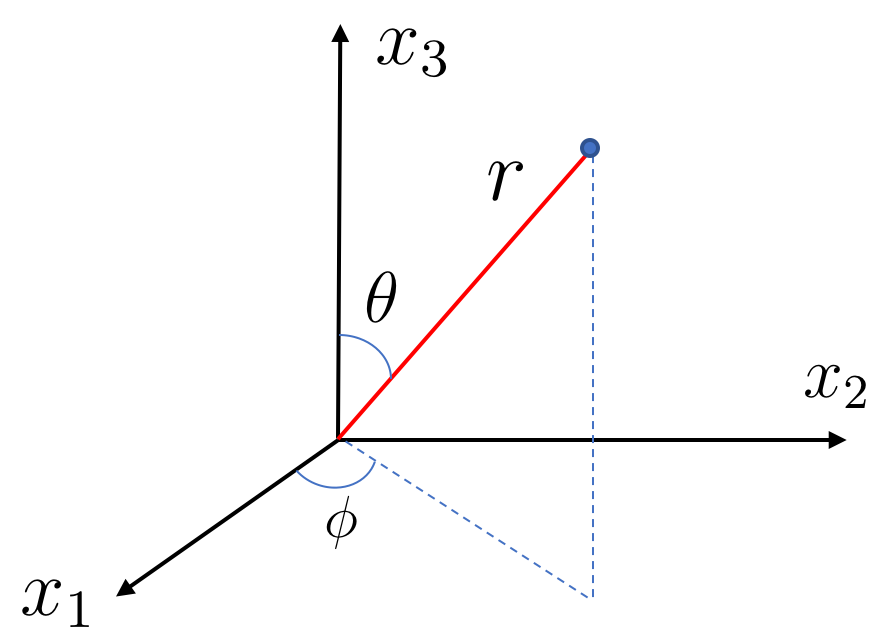
Our next task is to figure out the eigenfunctions and eigenvalues of the angular momentum operators . As you might expect, things become significantly simpler if we work in spherical polar coordinates. These are defined to be
| (4.91) | |||||
The relevant ranges of the angle are and as shown in the figure.
It’s straightforward to write the angular momentum operators in spherical polar coordinates. We just need to use the chain rule to get, for example,
with similar results for and .
Combining these, we can write the angular momentum operators as
| (4.92) |
Note that the angular momentum operators care nothing for how the wavefunctions depend on the radial coordinate . The angular momentum of a state is, perhaps unsurprisingly, encoded in how the wavefunction varies in the angular directions and . Furthermore, takes a particularly straightforward form, simply because is singled out as a special direction in spherical polar coordinates.
We also need an expression for the total angular momentum operator. This can be written most simply as
| (4.93) |
Again, we should be careful in interpreting what this means. In particular, the first acts both on the in round brackets, and also on whatever function the operator hits.
Our goal is to find simultaneous eigenfunctions for and . We’ll ignore all dependence for now, and reconsider it in the following sections when we solve the Schrödinger equation. The eigenfunction is straightforward: we can take
| (4.94) |
for any function . The wavefunction is single valued in , meaning , only if is an integer. Using (4.92), we see that the corresponding eigenvalues are
We learn that the angular momentum in the direction is quantised in units of . So too, of course, is the angular momentum in any other direction. But, as we’ve stressed above, if we sit in an eigenstate of , then we can’t also sit in an eigenstate of for any direction other than the -direction, with .
Next we turn to the eigenvalue equation. We keep the ansatz (4.94) and look for solutions
Using our expression (4.93), this becomes
| (4.95) |
Solutions to this equation are a well-studied class of mathematical functions called as associated Legendre Polynomials. Their construction comes in two steps. First, we introduce an associated set of functions known as (ordinary) Legendre Polynomials, . These obey the differential equation
The , with are polynomials of degree . The eigenfunction solutions (4.95) are then associated Legendre polynomials , defined by
The corresponding eigenvalue is
Because is a polynomial of degree , you only get to differentiate it times before it vanishes. This means that the angular momentum is constrained to take values that lie in the range
The upshot of this analysis is that the simultaneous eigenstates of and are given by functions that are labelled by two integers, and with ,
These functions are called spherical harmonics are are given by
The corresponding eigenvalues are
The integer is called the total angular momentum quantum number (even though, strictly speaking, the total angular momentum is really .) The integer is called the azimuthal angular momentum.
The requirement that is simply telling us that the angular momentum in a any given direction (in this case ) can’t be more than the total angular momentum. When (or ) you should think of the object as having angular momentum as aligned (or anti-aligned) with the -axis. When , you should think of the angular momentum as aligned in some intermediate direction. Of course, all of these thoughts should be quantum thoughts: even when , if you measure that angular momentum in a perpendicular direction like then you’re not guaranteed to get zero. Instead there will be a probability distribution of answers centred around zero.
To build some intuition, here are some of the first spherical harmonics. The case is just a constant
This is the case when a particle has no angular momentum and, correspondingly, its wavefunction has no angular dependence. In the context of atomic physics, it is referred to as an s-wave. The next collection of spherical harmonics all have total angular momentum ,
In the context of atomic physics, these are called p-wave states. The next, collection are d-waves,
There are various ways to visualise spherical harmonics. For example, in Figure 17,we plot the absolute value as the distance from the origin in the direction. Taking the absolute value removes the dependence, so these plots are symmetric around the -axis. Alternatively, in Figure 18, we plot on the sphere, with the value denoted by colour.
4.2 Solving the 3d Schrödinger Equation
We now return to the Schrödinger equation which, for a particle moving in a 3d central potential, is
As we’ve seen, the symmetry of the problem strongly suggests that we work in spherical polar coordinates (4.91), in terms of which the Laplacian becomes
Crucially, the angular parts of the Laplacian are identical to the total angular momentum operator that we met in (4.93). This means that we can equally well write the Laplacian as
Now we can see the utility of working with angular momentum eigenstates. We look for solutions to the Schrödinger equation of the form
where the radial wavefunction. All of the angular dependence now sits in an eigenstate of . Substituting this into the Schrödinger equation, what looks like a complicated partial differential equation turns into a more straightforward ordinary differential equation
| (4.96) |
where the potential is replaced with the effective potential
We’ve met this effective potential before. It’s exactly the same as the effective potential that emerges when solving classical mechanics problems in a central potential. The additional term is called the angular momentum barrier. The only difference from our previous classical result is that the angular momentum is now quantised in units of .
Note that the azimuthal angular momentum quantum number doesn’t appear in the Hamiltonian. (Sadly for us, there is an “” sitting in both the kinetic term and in the effective potential, but this is the mass! Not the angular momentum quantum number. Sorry! The canonical name for both is . It’s rare that it leads to confusion precisely because the azimuthal quantum number doesn’t appear in the Hamiltonian.)
Because the energy doesn’t depend on the eigenvalue , it means that the energy spectrum for any particle moving in a central potential will always be degenerate, with multiple eigenstates all having the same energy. In contrast, the energy will usually depend on the total angular momentum . This means that we expect each energy eigenvalue to have
| (4.97) |
which comes from the different states with .
The effective Schrödinger equation (4.96) takes a very similar form to those that we solved in Section 2. The only slight difference is the more complicated kinetic term, together with some associated issues about the need for a finite wavefunction at . However, these issues notwithstanding, we’re now largely on familiar territory. In the rest of this section we’ll briefly look at some appetisers before, in Section 4.3, we turn to our main course: the hydrogen atom.
4.2.1 The 3d Harmonic Oscillator
The harmonic oscillator provides a particularly simple example of the 3d Schrödinger equation because we can solve it in either Cartesian or polar coordinates. In Cartesian coordinates, the Hamiltonian is
We see that the Hamiltonian just decomposes into three copies of the 1d harmonic oscillator: one for each direction. This means that we can just read off the energy spectrum from our earlier result (2.36). The spectrum of the 3d harmonic oscillator is given by
| (4.98) |
where
All of the subtleties lie in the degeneracy of the spectrum. The ground state has energy and is unique. But there are three excited states with energy associated to exciting the harmonic oscillator in the , or direction. There are then 6 states with energy , because we could excite one oscillator twice or two oscillators once each. In general, the degeneracy of the level is .
How does this look in polar coordinates? It’s best to work with the form of the Schrödinger equation (4.96) which is now
We’re now awash with various constants and life will be easier if we can get rid of a few. We make the same scaling (2.29) that we used for the 1d oscillator,
The Schrödinger equation then becomes
| (4.99) |
We’re going to solve it using the same kind of polynomial expansion that we used for the 1d harmonic oscillator. First, look at the large distance behaviour. Here the dominant terms are
Next, look at the behaviour near the origin . Here the dominant terms in the equation are
If we make the power-law ansatz , we find
Here we’ve discarded the second solution on the grounds that the resulting wavefunction diverges at the origin. Putting this together, our ansatz for the general solution is
where we take
At this stage we’ve got a little bit of algebra to do, plugging our ansatz into the Schrödinger equation (4.99). Once the dust settles, you’ll find the result
| (4.100) |
We start our recursion relation by setting
This is just the statement that the small behaviour is indeed rather than some higher power. Now note that the first term in our equation will have term proportional to . But there’s nothing to cancel this in the second term. This means that we must set
As we’ll see, our recursion relation will then set for all odd . To find this recursion relation, we shift the summation variable in the first term in (4.100) so that all terms have the same power of ,
For this to hold for all , we must have the following recursion relation
At this stage, the argument is the same as we used for the 1d harmonic oscillator. If the recursion relation fails to terminate then for large , but that’s bad: it messes up the behaviour at large and turns it into a non-normalisable behaviour. This means that we must find solutions where the recursion relation terminates. This immediately allows us to read off the energy. If we are to have (recall that all for odd already vanish) then the energy of the state must be
| (4.101) |
Let’s compare this to our Cartesian result (4.98). Clearly they agree, but the extra work we did in polar coordinates brings more information: it tells us how the energy depends on the total angular momentum . In particular, the lowest energy state with angular momentum has .
We also have a better understanding of the degeneracy of states. When is even, the states with energy comprise of all even angular momentum states . Since there are states (4.97) associated to each angular momentum , the total number of states at level must be
which agrees with the count from the Cartesian calculation. Similarly, when is odd the states at energy comprise of all odd angular momentum states : again, the total count is .
4.2.2 Bound States in 3d
It is simple to adapt our earlier discussions to understand bound states in 3d. Here we’ll be brief as there is only one small punchline that we want to reach.
Consider the spherical finite potential well,
Clearly this is the 3d version of the 1d finite well that we considered in Section 2.3. The associated 3d radial Schrödinger equation (4.96) is
Our strategy is to massage the Schrödinger equation into the same form we saw in 1d and then simply invoke some of our earlier results. The only thing we need to fix is the unusual looking derivative terms. But this is easily achieved: we redefine the radial wavefunction as
| (4.102) |
Then, written in terms of the new function , the Schrödinger equation takes the 1d form
| (4.103) |
However, we haven’t quite washed away all traces of our 3d origin. Some remnant survives in the boundary conditions that we must impose on . First, the wavefunction must be normalisable. Since the ’s don’t cause us any trouble, we’re left with the requirement
where the factor in the middle equation comes from the integration measure for polar coordinates. We see that the normalisability condition restricts the asymptotic behaviour of as it would for a 1d wavefunction. The only novelty is what happens at the origin . Since is finite at the origin, clearly we need
| (4.104) |
The derivative must then be finite.
There is a simple fix to both these issues. We solve the Schrödinger equation (4.103) pretending that , defining . But we then look for odd solutions with
This condition ensures that we have as required. Moreover, we’re not missing any solutions. As we saw in Section 2, with an even potential all solutions are either even or odd, but the even solutions have and so are illegitimate for our present purposes.
This is all we need. We solved for the parity odd solutions in Section 2.3.1. In contrast to the parity even solutions, their existence is not guaranteed. They only arise when the potential is suitably deep or suitably wide, meaning (2.45)
This is our minor punchline. In 1d, there are potentials (like the finite well) where a bound state is always guaranteed. This is no longer the case in 3d where very shallow potentials do not house bound states.
Perhaps surprisingly, the case of turns out to be that same as with bound states guaranteed for certain classes of potentials, no matter how shallow. It is only in that you need a deep, wide potential to trap a quantum particle.
4.3 The Hydrogen Atom
The hydrogen atom is the simplest of all atoms. It consists of a single electron orbiting a proton, held in place by the Coulomb force
Here the electron has charge and the proton charge . The constant is a way to characterise the strength of the electrostatic force. For now, we’ll give values for neither nor but we’ll return to this after we’ve computed the energy spectrum. The associated Coulomb potential is
Our task in this section is to solve the 3d Schrödinger equation with this potential.
Following our discussion earlier in this section, we know that solutions will be characterised by three integers, , and , such that:
-
•
labels the energy state. We will take it run from . In the context of the hydrogen atom it is sometimes called the principal quantum number..
-
•
labels the total angular momentum. It appears in the eigenvalue of as .
-
•
labels the azimuthal angular momentum, also known as the angular momentum in the direction. It appears as the eigenvalue of .
We look for wavefunctions of the form
The Schrödinger equation (4.96) for the hydrogen atom is then given by,
where is the electron mass (and the subscript helps avoid confusion with the azimuthal angular momentum). Before we get going, let’s introduce some new variables so that we don’t have to lug around all those constants on our journey. We write
| (4.105) |
In this second of these redefinitions, we’ve anticipated the fact that we’re looking for negative energy bound states of the Coulomb potential, so that . You can check that has dimension of length. This cleans up the Schrödinger equation a little, which now reads
| (4.106) |
All we have to do now is solve it.
4.3.1 The Energy Spectrum
First, let’s look at the asymptotic behaviour of solutions as . Here the Schrödinger equation (4.106) is dominated by
We see that , which recall is related to the inverse energy of the system, sets the characteristic size of the wavefunction. Meanwhile, near the origin the dominant terms are
This is the same equation that we got when studying the 3d harmonic oscillator in Section 4.2. If we make the power-law ansatz , we find
where we’ve again discarded the second solution because it results in a wavefunction that diverges at the origin.
All of this motivates us to look for solutions of the form
| (4.107) |
where is a polynomial
| (4.108) |
where we must have so that we get the right behaviour at small .
Now we’ve got to roll up our sleeves and substitute this into the Schrödinger equation to get a recursion relation for the coefficients . It’s best to go slowly. First you can check that if you plug the ansatz (4.107) into (4.106), then the function must satisfy
Next, substitute the power-law ansatz (4.108) into this differential equation to find
Finally, shift the dummy summation variable in the second term to get a uniform power of . This then gives us our desired recursion relation
| (4.109) |
The argument that we now make follows that of the harmonic oscillator. Suppose that this recursion relation fails to terminate. Then, as , we have
But, as we explained in Section 2.2, this is the kind of expansion that we get from exponentially divergent functions of the form . On a mathematical level, there’s nothing wrong with these solutions: they just change the asymptotic form of (4.107) from to . But we’ve no use of such solutions for physics because they’re badly non-normalisable.
This means that, once again, we need to restrict attention to series that terminate. Which, in turn, means that there should be a positive integer for which , while for all . Clearly this holds only if takes special values,
Alternatively, since both and are integers, we usually define the integer
which obviously obeys . We then have
All that’s left is to chase through the definition of the various variables in this expression. These can be found in (4.105). The length scale is related to the energy scale which is given by
| (4.110) |
This is our final result for the energy spectrum of the hydrogen atom. The integer coincides with what we previously called the principal quantum number.
There’s a whole lot to unpick in this expression. First, there’s the ugly morass of constants sitting on the right-hand side. Clearly they set the energy scale of the bound states. There’s actually a better way to organise them to see what’s going on. To this end, we introduce the fine structure constant,
At first glance, you may think that this doesn’t help matters because, rather than simplifying things, we’ve introduced a new physical constant , the speed of light. However, the advantage of the fine structure constant is that it’s a dimensionless quantity. As you can see, it includes the expression familiar from the Coulomb force and it should be viewed as the convention-independent way to characterise the strength of electromagnetism. Moreover, it takes a value that’s easy to remember:
Written in terms of the fine structure constant, the energy eigenvalues are
This makes it clear what’s really setting the energy scale of the hydrogen atom: it is the rest mass energy of the electron! This is given by
A million electronvolts is an energy scale of relativistic particle physics. It is much larger than the typical energy scales of atomic physics but we can see why: there are two powers of the fine structure constant that interpolate between the two. The energy scale of the hydrogen atom is set by
This is called the Rydberg. As you can see, the (negative) ground state energy of the hydrogen atom is exactly one Rydberg; the higher excited states have energy . Note that the hydrogen atom has an infinite number of negative energy bound states.
Next there’s a surprise. The energy spectrum of hydrogen does not depend on the angular momentum . At least, that’s almost true: it depends only in the sense that the states for a given energy only include angular momentum . We saw a similar phenomenon for the 3d harmonic oscillator in Section 4.2 and this might lead you to think that this is common. It’s not. In fact, the only two systems where the energy spectrum doesn’t explicitly depend on angular momentum are the harmonic oscillator and the hydrogen atom!
The angular momentum does affect the degeneracy of the spectrum. Recall that there are states (4.97) associated to each total angular momentum . These are the states labelled by . For a fixed energy level , we can have any total angular momentum . This means that the degeneracy at level of the state at level is
The ground state is unique: it sits in s-wave. There are four excited states corresponding to the s-wave and three states of the p-wave. There are nine excited states, corresponding to the s-wave, the three p-wave states and five d-wave states. And so on.
The energy spectrum (4.110) is not quite the end of the story for the hydrogen atom. There are corrections due to special relativity. These corrections split the degeneracy so that the states with different , but the same , have different energies. These splitting are of order , much smaller than the original energies that are of order , and are referred to as the fine structure of the hydrogen atom. (In fact, this is where the name “fine structure constant” comes from.) You can read about these corrections in the lectures on Topics in Quantum Mechanics where we also start to explore multi-electron atoms and how to build up the periodic table of elements.
4.3.2 The Wavefunctions
The recursion relation (4.109) allows us to easily construct the corresponding wavefunctions. A state with energy has a wavefunction
where and is a polynomial of degree , defined by
with
These are known as generalised Laguerre polynomials. They are more conventionally written as .
The ground state wavefunction sits necessarily has vanishing angular momentum. It is simply
where the coefficient in front is chosen to normalise the wavefunction and the size of the wavefunction is given by
| (4.111) |
This is the Bohr radius. It sets the characteristic size of the hydrogen atom.
To get some sense for the wavefunctions, we’ve plotted the s-wave states for to in Figure 19. Note that each successive higher energy state contains an additional node. In Figure 20 we’ve fixed the energy level to and plotted successive higher angular momentum modes. This time we lose a node each time that increases.
For any wavefunction in the energy level, the peak can be approximated by writing , corresponding to a probability distribution . This has a maximum when , or
We see that the spatial extent of the higher energy states grows roughly as .
4.4 A Pre-Quantum Quantum History
The formalism of quantum mechanics that we have seen in these lectures was laid down in a flurry of creativity in the years 1925 and 1926. The primary builders of this new theory were Werner Heisenberg, Erwin Schrödinger, Max Born, Pascual Jordan, and Paul Dirac, several of them under the watchful grandfatherly eye of Niels Bohr.
The emergence of quantum mechanics was preceded by a quarter of a century of confusion, a time in which it was known that some old classical ideas must be jettisoned to explain various experiments, but it was far from clear what should replace them.
With hindsight, the first clear hint of the need for quantum mechanics came from the spectral lines of hydrogen. Take a tube filled with hydrogen gas and pass a current through it. The gas will glow but emit light only at very particular frequencies. In 1885, a Swiss school teacher called Johann Balmer noted that the wavelengths of the most prominent visible lines, shown in Figure 21, could be fitted to the formula
for (the red line), 4,5,6 and 7. Later Rydberg generalised this to the formula
which coincides with the Balmer formula when . Here is known as the Rydberg constant. The more prominent lines appear only in the UV are were not known to Balmer.
We now know that whenever integers appear in the laws of physics, they signify some underlying quantum effect. Indeed, the Rydberg formula follows straightforwardly from the spectrum of the hydrogen atom which, as we’ve seen, takes the form
| (4.112) |
If an electron sits in an excited state and drops to a lower state , , it will emit a photon with energy
The wavelength is related to the frequency by , so this immediately reproduces the Rydberg formula with
Of course, going backwards from the answer (4.112) is easy. But, in the early 1900’s, it was far from clear what to make of the Rydberg formula.
4.4.1 The Bohr Model
An important halfway house was provided by Bohr in 1913. This was only two years after Rutherford had shown that the atom consists of a tiny nucleus, with the electrons in remote orbits. Bohr took a collection of simple classical results and meshed them together with some quantum handwaving in a forced and somewhat unnatural manner to arrive at a remarkably accurate picture of the hydrogen atom. Here is his argument.
We start with the Coulomb force between an electron and proton
We assume that the electron orbits the proton on a classical trajectory that we take to be a circe. The Coulomb force must give the requisite centripetal force,
From this, we can determine the radius of the orbit in terms of the angular momentum ,
Similarly, the total energy can also be expressed in terms of the angular momentum
Now comes the quantum handwaving. Bohr postulated that angular momentum cannot take any value, but only integer amounts
This implies that the energy is quantised to take values
| (4.113) |
Remarkably, this is exactly the same as our exact result (4.112) from solving the Schrödinger equation. Furthermore, the minimum orbit of the electron is , given by
This is the Bohr radius; it also made an appearance as the size of our wavefunctions (4.111).
What’s going on here? There is clearly much that is wrong with the Bohr model. It assumes a classical trajectory which is far from the picture we now have of electrons as smeared clouds probability. It makes the wrong assumption for the quantisation of angular momentum, guessing that rather than, as we now know, . It also gets the connection between angular momentum and energy wrong; the correct answer should be . And yet, the end result (4.113) is miraculously exactly right! How can this be?
A pretty good answer to this question is simply: dumb luck. The hydrogen atom is unique among quantum systems in that these simple minded half-classical, half-quantum approaches give the right answers to certain important questions, most notably the energy spectrum. It’s not, however, a lesson that we can take and use elsewhere. In all other cases, to get the exact quantum result you have to do the hard work of solving the Schrödinger equation. The one exception to this is for the highly excited states, where Bohr’s kind of simple minded arguments do often provide a useful caricature of the physics. (For example, when the angular momentum is large there is not much difference between and .)
In fact, this same dumb luck arose earlier in the history of physics, although it was not realised at the time. Rutherford figured out the structure of the atom by interpreting the scattering of alpha particles off the nucleus. In particular, he derived a formula for the probability that an alpha particle would be deflected by some angle. (We derived Rutherford’s formula in the lectures on Dynamics and Relativity.) Of course, he derived this formula using classical mechanics even though we now know that classical mechanics is not a valid description for this scattering: one should use quantum mechanics. Here too, something miraculous occurs. The scattering formulae coming from quantum mechanics are typically very different from those derived using classical mechanics. There is just one exception: for the hydrogen atom, the two results coincide! The full quantum result will be calculated in the lectures on Topics in Quantum Mechanics.
We do, in fact, have a little better understanding of why the hydrogen atom is so special. It turns out that many of these seemingly miraculous properties can be traced to the existence of an extra operator that commutes with , and . This is called the Runge-Lenz vector. We won’t discuss it further in these lectures.
4.4.2 What About the Photon?
Much of the early history of quantum mechanics revolves around an object that we have barely mentioned in these lectures: the photon.
The first equation of quantum mechanics was proposed, somewhat unwittingly and, in later life begrudgingly, by Max Planck in his study of so-called blackbody radiation. This is the silly name given to the colour of light emitted by a hot object. The classical theory of Maxwell seemed to give nonsensical answers. Planck was able to derive a formula that agreed well with experiment but, buried with his derivation, was the suggestion that light comes in packets with energy given by
| (4.114) |
where is the (angular) frequency of light and is its wavelength. We already invoked this formula in our discussion of the spectral lines of hydrogen: it is used to relate the wavelength of emitted light to the difference in energy levels. You can read about the derivation of Planck’s blackbody radiation formula in the lectures on Statistical Physics.
Soon after Planck’s work, the formula (4.114) was put to good use by Einstein in his explanation of the photoelectric effect. If you shine a light on a metal, electrons are emitted. The surprise is that the electrons are emitted only if the frequency, rather than the intensity, of the light is sufficient.. If the frequency is a below a critical value, , then no electrons will be emitted no matter how strong the light. We now know that this occurs because the light is made of photons, each of energy . Any individual photon can dislodge an electron only if . If the frequency is too low, none of the photons can do the job.
We have met equations very similar to (4.114) in these lectures. For example, a stationary state has time dependence and energy . Furthermore, a non-relativistic particle with momentum has an associated de Brogle wavelength
These all gel nicely with the formula (4.114) if we further invoke the relativistic energy-momentum relation for a photon.
However, although we can get by with these simple minded formulae for a photon, it’s somewhat tricky to go any further. For example, we can’t easily write down an analog of the Schrödinger equation for the photon. The reason can, at heart, be traced to the factor of in (4.114). Anywhere the speed of light appears, we really dealing with special relativity. There is a formulation of quantum mechanics that is fully compatible with special relativity: it goes by the name of quantum field theory. For example, this framework allows us to start with the Maxwell equations of electromagnetism and derive the Planck formula (4.114), rather than postulate it as a further axiom. We will see how to do this when we come to study Quantum Field Theory.
4.5 A First Look at Renormalisation
There is a scene in the movie Back to the Future where Marty McFly introduces the unsuspecting audience at the Enchantment Under the Sea dance to a little bit of rock and roll. Things start off pretty well. Then he gets carried away. As the song finishes, Marty opens his eyes to see a stunned, silenced audience staring back at him and sheepishly admits “I guess you guys aren’t ready for that yet…but your kids are going to love it.”
This section is our Enchantment Under the Sea moment. We will discuss the topic of renormalisation. You should be aware that this is a ridiculously inappropriately advanced topic to include in introductory lectures on quantum mechanics. Chances are you guys aren’t ready for it yet. But your future selves are going to love it.
What is Renormalisation?
The topic of renormalisation usually only arises when we discuss quantum field theory. It is, moreover, a topic that is woefully described in various popular science accounts, all of which seem to be rooted in a 1950s view of the world.
The topic starts with the observation that quantum field theory is hard. In these lectures we’ve found various exact solutions to the Schrödinger equation. That’s a luxury that we no longer have when it comes to the more interesting classes of quantum field theories. Instead, if we want to solve them we must develop approximation techniques and the simplest of these goes by the name of perturbation theory. This means that we start by finding an approximate solution to the problem and then systematically improve matters by adding increasingly small corrections, not unlike a Taylor series approximation to a function.
In the early days of quantum field theory, the first stab at the solution gave pretty impressive results. But the successive improvements were a disaster. They all gave the answer infinity. Needless to say, it’s difficult to view infinity as a small correction to the original answer.
A solution of sorts was found in the 1950s by Tomonaga, Schwinger and Feynman, and synthesised by Dyson. Their solution can be paraphrased by the following equation
In other words, they found a way to subtract an infinity from the original infinity to leave behind an unambiguous, finite answer. Physically, the results were nothing short of spectacular. The calculations gave agreement between theory and experiment to many significant figures. However, the technique left a lot to be desired. Why should we be forced to resort to such mathematical nonsense as subtracting one infinity from another?
A physical understanding of renormalisation came only in the 1970s, primarily through the work of Kenneth Wilson. First he showed that, despite appearances, renormalisation has nothing to do with physical infinities. Indeed, viewed the right way, there are no infinities in quantum field theory. They arose in the earlier calculations because theorists implicitly assumed that their theories should hold to arbitrarily small distance scales. A little humility, and an acceptance that we don’t yet know what’s happening on the very smallest distances, then serves to eliminate the infinity. Although it’s not immediately obvious, this perspective on renormalisation has a striking consequence: it turns out that the constants of nature depend on the distance scale at which they’re measured.
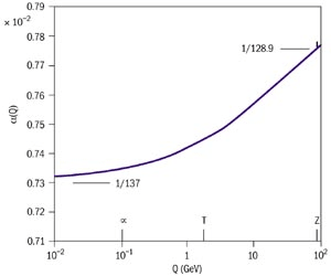
For example, we’ve already met the fine structure constant that characterises the strength of the electromagnetic force. It is roughly
Strictly speaking, however, we should say that asymptotes to this value at distance scales larger than metres. Of course, most experiments that we do involving electromagnetism take place on scales much larger than this which is why we always quote the value. But when it comes to to the realm of particle physics, we routinely probe distances smaller than m. And when we do, we see that starts to increase. The experimental data is shown in the figure, with plotted on the vertical axis and the log of the inverse distance plotted on the horizontal axis (). You can read more about a cartoon version of renormalisation in the lectures on Particle Physics. You can learn about the details of Wilson’s approach to renormalisation in the lectures on Statistical Field Theory.
By the time you get to quantum field theory, it’s difficult to ignore renormalisation. In the world of non-relativistic quantum mechanics, however, you need to seek it out. Happily there is a simple quantum mechanical example that exhibits many of the features of renormalisation, but in a setting where we can happily understand what’s going on using nothing more than the Schrödinger equation.
4.5.1 A Delta Function Potential in the Plane
We consider a particle moving on the plane with a delta function potential at the origin
The delta function is taken with a negative sign and so that it is attractive. The Schrödinger equation is
We solved the corresponding problem in 1d in Section 2.3.2 without a hitch. There we found that there was precisely one bound state localised around the delta function. We’ll now see that things are significantly more subtle in 2d. We’ll first argue that there can be no bound states in a 2d delta function. We’ll then look a little more closely and see that, when viewed the right way, the 2d delta function does admit a bound state after all.
First, note that the 2d problem has a surprising property. If we define
then the Schrödinger equation becomes
| (4.115) |
To proceed, let’s do some dimensional analysis. Suppose that we generalise the above problem to a particle moving in spatial dimensions. The kinetic term always has dimensions of (length) while the delta function has dimensions of (length) because you integrate it over to get the number one. This picks out spatial dimensions as special because only there do and both have dimensions of (length).
This has consequence. First, it would seem to preclude the possibility of bound states. Such a bound state would have some negative energy
But what could be? The only parameter is but this is dimensionless, while has dimension of (length). There’s simply no scale in the problem that could set a value for .
Another way of saying this is to note that the Schrödinger equation has a novel symmetry. Suppose that we find a solution, whether a bound state with negative energy or a state that can be interpreted as in terms of scattering with . We then rescale the spatial coordinates
The Schrödinger equation becomes
If solves the Schrödinger equation with energy then solves the Schrödinger equation with energy . In other words, there is a continuum of states. This is to be expected for scattering states with positive energy: asymptotically these states look like . But it’s not what we expect for bound states with negative energy. In particular, it would mean that there are bound states of arbitrarily negative energy.
This all sounds like a very good reason to discount the possibility of bound states in this problem. That would certainly avoid all the issues mentioned above. In fact, as we now see, the truth is significantly more interesting.
We will solve the Schrödinger equation with a flurry of Fourier transforms. We write the wavefunction as
| (4.116) |
We then substitute this Fourier transform only in the and terms of (4.115) to get
where, on the right-hand side we’ve replaced on account of the fact that this is the only value the delta function sees. Now, we use the Fourier transform once again, but this time for the delta function itself, which can be written as
This gives us
Finally, we multiply both sides by and integrate over ,
This is a clever thing to do as everything now simplifies. The integral over gives us a delta function
which then, in turn, kills the integral over on the left-hand side. We’re left with the simple equation
This looks like we’ve done our job. The bound state solutions with energy have Fourier coefficients
| (4.117) |
The value is an arbitrary constant which, for a bound state, should be non-zero as this is the only thing the delta function knows about. We can now do a consistency check. The value of is also given by our original Fourier transform (4.116),
We can compare this with the integral of (4.117): we get
| (4.118) |
We don’t care about the value of in this equation: just that it’s non-vanishing. Instead, (4.118) should be viewed as an integral equation to determine the bound state energy . If you evaluate the equivalent integral for the 1d delta function, you’ll reproduce our earlier answer (2.47) which is satisfying. But for the 2d delta function there’s a problem because the integral does not converge. It is given by
| (4.119) |
This is entirely analogous to the infinities that were encountered in the early days of quantum field theory. Of course, in the present context we could simply shrug and say “see, I told you there should be no bound states”. But our quantum field theoretic forefathers didn’t have this option and we can learn from their perseverance.
4.5.2 Renormalisation in Quantum Mechanics
To make sense of the in the integral (4.119), let’s first render it finite. We do this by changing the integral
Here is called the UV-cut off. It “cuts off” the integral at high , where the Fourier modes oscillate on very small distance scales. (The name “UV-cut off” is a quaint nod to the idea that UV light also has a high frequency. Admittedly, if the analogy was in anyway accurate it would be called “gamma-ray cut-off”, but the term UV has stuck.)
What physical motivation do we have for changing the integral in this way? Well, one answer might be that we’re not entirely sure that our original quantum mechanical model was correct. After all, we included an infinitely thin delta function potential which doesn’t sound particularly realistic. In most situations, delta function potentials are introduced as a simple toy model to capture the key physics and their infinitely spikey nature should not be taken too seriously. But, if this is the reason that we’re studying the delta-function then it doesn’t bode particularly well for trusting our theory when it comes to very short distance scales.
The introduction of the UV cut-off should be thought of as an injection of humility into the proceeding. The UV cut-off is simply an expression of our ignorance of what’s going on at short distance scales. The rub is that no physical property can depend on our ignorance. That means that, somehow, must drop out of any final answer that we submit.
Let’s see how we do. Our consistency condition (4.118) becomes
Rearranging, we find the bound state energy
| (4.120) |
At first glance, it doesn’t look like this is much of an improvement. First, the bound state energy explicitly depends on the UV cut-off. Moreover, as we send to recover the original theory, we see that the bound state energy disappears off to infinity. Once again, all signs suggest that our delta function doesn’t have a bound state.
Now we introduce the key idea: the dimensionless coupling should also depend on the distance scale of the theory. In particular, if we change the UV cut-off then we should change also change at the same time. In fact, we see that we get to realise our dream of having the physical bound state energy independent of if we take
| (4.121) |
This is called the running of the coupling.
What’s going on here? It’s tempting to think that we can define a quantum theory by specifying a Hilbert space and a Hamiltonian, with various parameters set to specific values. That’s what we’ve done throughout these lectures, and it’s what we continue to do in nearly all problems in non-relativistic quantum mechanics. However, it turns out that it’s not the right way to think in quantum field theory and, perhaps surprisingly, it’s not the right approach with our 2d delta function either. Instead, the correct definition of the theory describing a particle moving in the presence of a two-dimensional delta function includes both a UV cut-off and a dimensionless coupling . From these two, we then get the bound state energy scale (4.120). Within this more generalised class of theories, the 2d delta function has a single bound state, just like its 1d counterpart.
However, and come together in a pair. They’re not independent. You can change the UV cut-off without changing the underlying theory by making a compensating change to the coupling constant. The formula (4.121) tells you how to do this.
The fact that the coupling varies with the cut-off also has physical implications. We could, for example, study scattering off the delta-function potential. With a cut-off in place, you will find that the probability for scattering at energy (captured in so-called phase shifts) will depend on . In other words, it appears as if the effective strength of the delta function varies in energy in the same way as the running of the coupling (4.121). This is entirely analogous to the energy dependent fine structure constant that we mentioned previously. We will discuss scattering in higher dimensions in the lectures on Topics in Quantum Mechanics, although we will steer clear of any discussion of renormalisation in that context.
Our previous arguments suggesting that a bound state cannot exist are all nullified by the presence of the UV cut-off. In particular, provides the dimensions necessary to set the energy scale of and breaks the scaling symmetry that we naively thought was a property of the Hamiltonian.
In fact, all of these previous arguments really took place in a theory in which we implicitly took while keeping fixed. This lead us to believe that there is no finite energy bound state. The formula (4.121) tells us what’s really going on: as we remove the cut-off, we can keep the finite energy bound state but only by sending as . We see that there is a delicate balancing act between these two parameters. An arbitrarily weak delta function can still lead to a finite energy bound state if we admit arbitrarily small wavelength modes in our theory.
Theories which have the property that some dimensionless parameter, like , vanishes as we go to higher and higher energies are said to be asymptotically free. In particle physics, the strong nuclear force, which is described by Yang-Mills theory, has this property.
It’s also worth looking at what happens in the limit of small . Here the formula for the bound state energy (4.120) is
| (4.122) |
This ensures that the energy scale of the bound state is way below the cut-off: . This is good! As we stressed above, the cut-off is a parameterisation of our ignorance. We should only trust physics on distance scales much bigger than or, equivalently, on energy scales much less than .
In fact, a better characterisation of (4.122) would be . For small , the function is really tiny. To get some sense of this, we could try to Taylor expand . The first term is zero. The next term is also zero. In fact, the Taylor expansion of vanishes identically because, for small the function is smaller than for any .
There a quite a few places in physics where two different energy scales are related by a small number of the form for some . Whenever this arises, it is always interesting. Prominent examples include how electrons pair up in superconductors, how quarks bind together into protons and neutrons, and how D-branes emerges in string theory. There is a whole lot of physics goodness in these ideas that we will come to in future courses.